In this post, we are going to diving into the Spring framework in deep. The main content of this post is to analyze IoC implementation in the source code of the Spring framework.
Basics
Basic Concepts
Bean and BeanDefinition
In Spring, the objects that form the backbone of your application and that are managed by the Spring IoC container are called beans. A bean is an object that is instantiated, assembled, and otherwise managed by a Spring IoC container.
A Spring IoC container manages one or more beans. These beans are created with the configuration metadata that you supply to the container, for example, in the form of XML <bean/> definitions.
Within the container itself, these bean definitions are represented as BeanDefinition objects.
BeanWrapper
BeanWrapper is the central interface of Spring’s low-level JavaBeans infrastructure. Typically not used directly but ranther implicitly via a BeanFactory or a DataBinder. It provides operations to analyze and manipulate standard JavaBeans: get and set property values, get property descriptors, and query the readability/writability of properties.
IoC Containers
IoC container is the implementation of IoC functionality in the Spring framework. The interface org.springframework.context.ApplicationContextrepresents the Spring IoC container and is responsible for instantiating, configuring, and assembling the aforementioned beans. The container gets its instructions on what objects to instantiate, configure, and assemble by reading configuration metadata. The configuration metadata is represented in XML, Java annotations, or Java code. It allows you to express the objects that compose your application and the rich interdependencies between such objects.
Several implementations of the ApplicationContext interface are supplied out-of-the-box with Spring. In standalone applications it is common to create an instance of ClassPathXmlApplicationContext or FileSystemXmlApplicationContext.
BeanFactory vs ApplicationContext
Spring provides two kinds of IoC container, one is XMLBeanFactory and other is ApplicationContext. The ApplicationContext is a more powerful IoC container than BeanFactory.
Bean Factory
Bean instantiation/wiring
Application Context
Bean instantiation/wiring
Automatic BeanPostProcessor registration
Automatic BeanFactoryPostProcessor registration
Convenient MessageSource access (for i18n)
ApplicationEvent publication
WebApplicationContext vs ApplicationContext
WebApplicationContext interface provides configuration for a web application. This is read-only while the application is running, but may be reloaded if the implementation supports this.
WebApplcationContext extends ApplicationContext. This interface adds a getServletContext() method to the generic ApplicationContext interface, and defines a well-known application attribute name that the root context must be bound to in the bootstrap process.
WebApplicationContext in Spring is web aware ApplicationContext i.e it has Servlet Context information. In single web application there can be multiple WebApplicationContext. That means each DispatcherServlet associated with single WebApplicationContext.
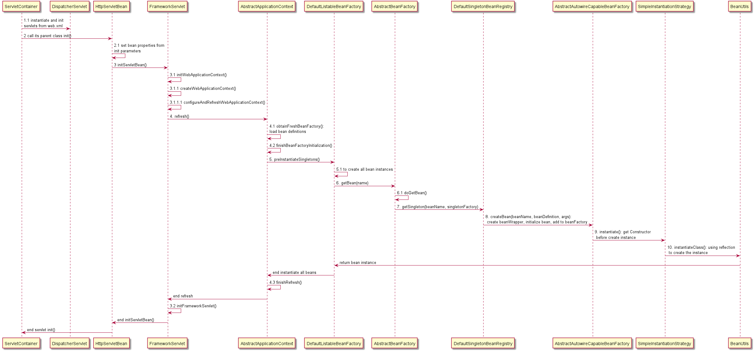
The following figure shows the process of IoC implementation.
Next, We are going to analyze the implementation in the source code of every step.
1 Java web project starting
1.1 instantiate and init servlets from web.xml
When a Java web project running in an application server like Apache Tomcat, the servlet container of the server will load, instantiate, and init Java servlets that be <load-on-startup> from web.xml file.
As this is a startup method, it should destroy already created singletons if it fails, to avoid dangling resources. In other words, after invocation of that method, either all or no singletons at all should be instantiated.
AbstractApplicationContext.java
publicvoidrefresh()throws BeansException, IllegalStateException { //... // 1. Create a BeanFactory instance. Refer to #4.1 ConfigurableListableBeanFactorybeanFactory=this.obtainFreshBeanFactory(); // 2. Configure properties of AbstractApplicationContext, prepare for bean initialization and context refresh this.postProcessBeanFactory(beanFactory); this.invokeBeanFactoryPostProcessors(beanFactory); this.registerBeanPostProcessors(beanFactory); this.initMessageSource(); this.initApplicationEventMulticaster(); this.onRefresh(); this.registerListeners(); // 3. bean initialization. Refer to #4.2 this.finishBeanFactoryInitialization(beanFactory); // 4. context refresh. this.finishRefresh(); // ... }
4.1 obtainFreshBeanFactory()
Create a BeanFactory instance in AbstractRefreshableApplicationContext.
AbstractRefreshableApplicationContext.java
protectedfinalvoidrefreshBeanFactory()throws BeansException { //... // 1. Creating a BeanFactory instance. DefaultListableBeanFactorybeanFactory=this.createBeanFactory(); // 2. Set BeanFactory instance's properties beanFactory.setSerializationId(this.getId()); this.customizeBeanFactory(beanFactory); // 3. load bean definitions this.loadBeanDefinitions(beanFactory); // 4. assign this new BeanFactory instance to the AbstractRefreshableApplicationContext's field beanFactory synchronized(this.beanFactoryMonitor) { this.beanFactory = beanFactory; } //... }
// 1. check is the bean instance in creation if (sharedInstance != null && args == null) { //... } else { // 2. get and check beanDefinition by beanName RootBeanDefinitionmbd=this.getMergedLocalBeanDefinition(beanName); this.checkMergedBeanDefinition(mbd, beanName, args); // 3. to get different type bean instance: singleton, prototype, and so on. if (mbd.isSingleton()) { // to create singleton bean instance go to #7 sharedInstance = this.getSingleton(beanName, () -> { try { returnthis.createBean(beanName, mbd, args); } catch (BeansException var5) { this.destroySingleton(beanName); throw var5; } }); bean = this.getObjectForBeanInstance(sharedInstance, name, beanName, mbd); } elseif (mbd.isPrototype()) { //... } else{ //... } } }
7 getSingleton(beanName, singletonFactory) in DefaultSingletonBeanRegistry
To get singleton bean instance.
DefaultSingletonBeanRegistry.java
public Object getSingleton(String beanName, ObjectFactory<?> singletonFactory) { // 1. check conditions and logging //... // 2. to get a singleton bean instance, go to #8 singletonObject = singletonFactory.getObject(); newSingleton = true; // 3. add created singleton bean instance to the bean list if (newSingleton) { this.addSingleton(beanName, singletonObject); } }
protectedvoidaddSingleton(String beanName, Object singletonObject) { synchronized(this.singletonObjects) { // add bean instance to the bean list "singletonObjects" this.singletonObjects.put(beanName, singletonObject); this.singletonFactories.remove(beanName); this.earlySingletonObjects.remove(beanName); this.registeredSingletons.add(beanName); } }
8 createBean(beanName, beanDefinition, args) in AbstractAutowireCapableBeanFactory
To get a bean instance, create a beanWrapper, initialize the bean, add add the bean to the beanFactory.
AbstractAutowireCapableBeanFactory.java
protected Object createBean(String beanName, RootBeanDefinition mbd, @Nullable Object[] args)throws BeanCreationException { // ... // 1. construct a beanDefinition for use. // ... // 2. try to create bean instance ObjectbeanInstance=this.resolveBeforeInstantiation(beanName, mbdToUse); if (beanInstance != null) { return beanInstance; } // 3. try to create bean instance again if fail to create in first time beanInstance = this.doCreateBean(beanName, mbdToUse, args); return beanInstance; }
protected Object doCreateBean(String beanName, RootBeanDefinition mbd, @Nullable Object[] args)throws BeanCreationException { // 1. to construct a beanWrapper and create the bean instance BeanWrapperinstanceWrapper=this.createBeanInstance(beanName, mbd, args); // 2. post processing //... // 3. Add bean to the beanFactory and some bean instances record list this.addSingletonFactory(beanName, () -> { returnthis.getEarlyBeanReference(beanName, mbd, bean); }); // 4. autowired and handle property values this.populateBean(beanName, mbd, instanceWrapper); // 5. initialization bean exposedObject = this.initializeBean(beanName, exposedObject, mbd); // 6. return bean return exposedObject; }
protected BeanWrapper instantiateBean(String beanName, RootBeanDefinition mbd) { // 1. to create the bean instance ObjectbeanInstance=this.getInstantiationStrategy().instantiate(mbd, beanName, this);
// 2. create the BeanWrapper by bean instance BeanWrapperbw=newBeanWrapperImpl(beanInstance); this.initBeanWrapper(bw); return bw; }
9 instantiate() in SimpleInstantiationStrategy
Get the Constructor of the bean class and to get the bean instance.
SimpleInstantiationStrategy.java
public Object instantiate(RootBeanDefinition bd, @Nullable String beanName, BeanFactory owner) { // 1. get the Constructor of the bean class ConstructorconstructorToUse= (Constructor)bd.resolvedConstructorOrFactoryMethod; Class<?> clazz = bd.getBeanClass(); constructorToUse = (Constructor)AccessController.doPrivileged(() -> { return clazz.getDeclaredConstructor(); }); // 2. to craete bean instance return BeanUtils.instantiateClass(constructorToUse, newObject[0]); }
10 instantiateClass() in BeanUtils
Using reflection to create a instance.
BeanUtils.java
publicstatic <T> T instantiateClass(Constructor<T> ctor, Object... args)throws BeanInstantiationException { //... // Using reflection to create instance return ctor.newInstance(argsWithDefaultValues); }
Conclusion
Spring framework uses the servlet container loads the DispatcherServlet when server startup to trigger the automatic beans instantiation.
The ApplicationContext is responsible for the whole process of beans instantiation. There is a BeanFactory as a field in the ApplicationContext, it is responsible to create bean instances.
The important steps of beans instantiation are: load bean definitions, create and initialize beanFactory, create and initialize bean instances, keep bean records in beanFactory.
Many applications perform well with the default settings of a JVM, but some applications require additional JVM tuning to meet their performance requirement. A well-tuned JVM configurations used for one application may not be well suited for another application. As a result, understanding how to tune a JVM is a necessity.
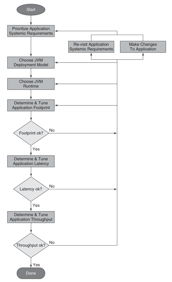
Process of JVM Tuning
The following figure shows the process of JVM tuning.
The first thing of JVM tuning is prioritize application systemic requirements. In contrast to functional requirements, which indicate functionally what an application computes or produces for output, systemic requirements indicate a particular aspect of an application’s such as its throughput, response time, the amount of memory it consumes, startup time, availability, manageability, and so on.
Performance tuning a JVM involves many trade-offs. When you emphasize one systemic requirement, you usually sacrifice something in another. For example, minimizing memory footprint usually comes at the expense of throughput and/or latency. As you improve manageability, you sacrifice some level of availability of the application since running fewer JVMs puts a larger portion of an application at risk should there be an unexpected failure. Therefore, when emphasizing systemic requirements, it is crucial to the tuning process to understand which are most important to the application.
Once you know which systemic requirements are most important, the following steps of tuning process are:
Choose a JVM deployment mode.
Choose a JVM runtime environment.
Tuning the garbage collector to meet your application’s memory footprint, pause time/latency, and throughput requirements.
For some applications and their systemic requirements, it may take several iterations of this process until the application’s stakeholders are satisfied with the application’s performance.
Application Execution Assumptions
An initialization phase where the application initializes important data structures and other necessary artifacts to begin its intended use.
A steady state phase where the application spends most of its time and where the application’s core functionality is executed.
An optional summary phase where an artifact such as a report may be generated, such as that produced by executing a benchmark program just prior to the application ending its execution.
The steady state phase where an application spends most of its time is the phase of most interest.
Testing Infrastructure Requirements
The performance testing environment should be close to the production environment. The better the testing environment replicates the production environment running with a realistic production load, the more accurate and better informed tuning decision will be.
Application Systemic Requirements
There are several application systemic requirements, such as its throughput, response time, the amount of memory it consumes, its availability, its manageability, and so on.
Availability
Availability is a measure of the application being in an operational and usable state. An availability requirement expresses to what extent an application, or portions of an application, are available for use when some component breaks or experiences a failure.
In the context of a Java application, higher availability can be accomplished by running portions of an application across multiple JVMs or by multiple instances of the application in multiple JVMs. One of the trade-offs when emphasizing availability is increased manageability costs.
Manageability
Manageability is a measure of the operational costs associated with running and monitoring the application along with how easy it is configure the application. A manageability requirement expresses the ease with which the system can be managed. Configuration tends to be easier with fewer JVMs, but the application’s availability may be sacrificed.
Throughput
Throughput is a measure of the amount of work that can be performed per unit time. A throughput requirement ignores latency or responsiveness. Usually, increased throughput comes at the expense of either an crease in latency and/or an increase in memory footprint.
Latency and Responsiveness
Latency, or responsiveness, is a measure of the elapsed time between when an application receives a stimulus to do some work and that work is completed. A latency or responsiveness requirement ignores throughput. Usually, increased responsiveness or lower latency, comes at the expense of lower throughput and/or an increase in memory footprint.
Memory Footprint
Memory footprint is a measure of the amount of memory required to run an application at a some level of throughput, some level of latency, and/or some level of availability and manageability. Memory footprint is usually expressed as either the amount of Java heap required to run the application and/or the total amount of memory required to run the application.
Startup Time
Startup time is a measure of the amount of time it takes for an application to initialize. The time it takes to initialize a Java application is dependent on many factors including but not limited to the number of classes loaded, the number of objects that require initialization, how those objects are initialized, and the choice of a HotSpot VM runtime, that is, client or server.
Rank Systemic Requirements
The first step in the tuning process is prioritizing the application’s systemic requirements. Doing so involves getting the major application stakeholders together and agreeing upon the prioritization.
Ranking the systemic requirements in order of importance to the application stakeholders is critical to the tuning process. The most important systemic requirements drive some of the initial decisions.
Choose JVM Deployment Model
There is not necessarily a best JVM deployment model. The most appropriate choice depends on which systemic requirements (manageability, availability, etc.) are most important.
Generally, with JVM deployment models has been the fewer the JVMs the better. With fewer JVMs, there are fewer JVMs to monitor and manage along with less total memory footprint.
Choose JVM Runtime
Choosing a JVM runtime for a Java application is about making a choice between a runtime environment that tends to be better suited for one or another of client and server applications.
There are several runtime environments to consider: client or server runtime, 32-bit or 64-bit JVM, and garbage collectors.
Client or Server Runtime
There are three types of JVM runtime to choose from when using the HotSpot VM: client, server, or tiered.
The client runtime is specialized for rapid startup, small memory footprint, and a JIT compiler with rapid code generation.
The server runtime offers more sophisticated code generation optimizations, which are more desirable in server applications. Many of the optimizations found in the server runtime’s JIT compiler require additional time to gather more information about the behavior of the program and to produce better performing generated code.
The tiered runtime which combines the best of the client and server runtimes, that is, rapid startup time and high performing generated code.
If you do not know which runtime to initially choose, start with the server runtime. If startup time or memory footprint requirements cannot be met and you are using Java 6 Update 25 or later, try the tiered server runtime. If you are not running Java 6 Update 25 or later, or the tiered server runtime is unable to meet your startup time or memory footprint requirement, switch to the client runtime.
32-Bit or b4-Bit JVM
There is a choice between 32-bit and 64-bit JVMs.
The following table provides some guidelines for making an initial decision on whether to start with a 32-bit or 64-bit JVM. Note that client runtimes are not available in 64-bit HotSpot VMs.
Operating System
Java Heap Size
32-Bit or 64-Bit JVM
Windows
Less than 1300 megabytes
32-bit
Windows
Between 1500 megabytes and 32 gigabytes
64-bit with -d64 -XX:+UseCompressedOops command line options
Windows
More than 32 gigabytes
64-bit with -d64 command line option
Linux
Less than 2 gigabytes
32-bit
Linux
Between 2 and 32 gigabytes
64-bit with -d64 -XX:+UseCompressedOops command line options
Linux
More than 32 gigabytes
64-bit with -d64 command line option
Oracle Solaris
Less than 3 gigabytes
32-bit
Oracle Solaris
Between 3 and 32 gigabytes
64-bit with -d64 -XX:+UseCompressedOops command line options
Oracle Solaris
More than 32 gigabytes
64-bit with -d64 command line option
Garbage Collectors
There are several garbage collectors are available in the HotSpot VM: serial, throughput, mostly concurrent, and garbage first.
Since it is possible for applications to meet their pause time requirements with the throughput garbage collector, start with the throughput garbage collector and migrate to the concurrent garbage collector if necessary. If migration to the concurrent garbage collector is required, it will happen later in the tuning process as part of determine and tune application latency step.
The throughput garbage collector is specified by the HotSpot VM command line option -XX:+UseParallelOldGC or -XX:+UseParallelGC. The difference between the two is that the -XX:+UseParallelOldGC is both a multithreaded young generation garbage collector and a multithreaded old generation garbage collector. -XX:+UseParallelGC enables only a multithreaded young generation garbage collector.
GC Tuning Fundamentals
GC tuning fundamentals contain the following content: attributes of garbage collection performance, GC tuning principles, and GC logging. Understanding the important trade-offs among the attributes, the tuning principles, and what information to collect is crucial to JVM tuning.
The Performance Attributes
Throughput.
Latency.
Footprint.
A performance improvement for one of these attributes almost always is at the expense of one or both of the other attributes.
The Principles
There are three fundamental principle to tuning GC:
The minor GC reclamation principle. At each minor garbage collection, maximize the number of objects reclaimed. Adhering to this principle helps reduce the number and frequency of full garbage collections experienced by the application. Full GC typically have the longest duration and as a result are applications not meeting their latency or throughput requirements.
The GC maximize memory principle. The more memory made available to garbage collector, that is, the larger the Java heap space, the better the garbage collector and application perform when it comes to throughput and latency.
The 2 of 3 GC tuning principle. Tune the JVM’s garbage collector for two of the three performance attributes: throughput, latency, and footprint.
Keeping these three principles in mind makes the task of meeting your application’s performance requirements much easier.
Command Line Options and GC Logging
The JVM tuning decisions made utilize metrics observed from monitoring garbage collections. Collecting this information in garbage collection logs is the best approach. This garbage collection statistics gathering must be enabled via HotSpot VM command line options. Enabling GC logging, even in production systems, is a good idea. It has minimal overhead and provides a wealth of information that can be used to correlate application level events with garbage collection or JVM level events.
Several HotSpot VM command line options are of interest for garbage collection logging. The following is the minimal set of recommended command line options to use:
In the first line of GC logging, 46.152 is the number of seconds since the JVM launched.
In the second line, PSYoungGen means a young generation garbage collection. 295648K->32968K(306432K) means the occupancy of the young generation space prior and after to the garbage collection. The value inside the parentheses (306432K) is the size of the young generation space, that is, the total size of eden and the two survivor spaces.
In the third line, 296198K->33518K(1006848K) means the Java heap utilization before and after the garbage collection. The value inside the parentheses (1006848K) is the total size of the Java heap.
In the fourth line, [Times: user=1.83 sys=0.01, real=0.11 secs] provides CPU and elapsed time information. 1.83 seconds of CPU time in user mode, 0.01 seconds of operating system CPU time, 0.11 seconds is the elapsed wall clock time in seconds of the garbage collection. In this example, it took 0.11 seconds to complete the garbage collection.
Determine Memory Footprint
Up to this point in the tuning process, no measurements have been taken. Only some initial choices have been made. This step of tuning process provides a good estimate of the amount of memory or Java heap size required to run the application. The outcome of this step identifies the live data size for the application. The live data size provides input into a good starting point for a Java heap size configuration to run the application.
Live data size is the amount of memory in the Java heap consumed by the set of long-lived objects required to run the application in its steady state. In other words, it is the Java heap occupancy after a full garbage collection while the application is in steady state.
Constraints
The following list helps determine how much physical memory can be made available to the JVM(s):
Will the Java application be deployed in a single JVM on a machine where it is the only application running? If that is the case, then all the physical memory on the machine can be made available to JVM.
Will the Java application be deployed in multiple JVMs on the same machine? or will the machine be shared by other processes or other Java application? If either case applies, then you must decide how much physical memory will be made available to each process and JVM.
In either of the preceding scenarios, some memory must be reserved for the operating system.
HotSpot VM Heap Layout
Before taking some footprint measurements, it is important to have an understanding of the HotSpot VM Java heap layout. The HotSpot VM has three major spaces: young generation, old generation, and permanent generation. The heap data area composes of the young generation and the old generation.
The new objects are allocated in the young generation space. Objects that survive after some number of minor garbage collections are promoted into the old generation space. The permanent generation space holds VM and Java class metadata as well as interned Strings and class static variables.
Following command line options specify the size of area data space:
Heap area
-Xmx specified the maximum size of heap.
-Xms specified the initial size of heap.
Young generation
-XX:NewSize=<n>[g|m|k] specified the initial and minimum size of the young generation space.
-XX:MaxNewSize=<n>[g|m|k] specified the maximum size of the young generation space.
-Xmn<n>[g|m|k] sets the initial, minimum, and maximum size of the young generation space.
Permanent generation
-XX:PermSize=<n>[g|m|k] specified the initial and minimum size of permanent generation space.
-XX:MaxPermSize=<n>[g|m|k] specified the maximum size of permanent space.
If any Java heap size, initial or maximum size, young generation size, or permanent generation size is not specified, the HotSpot VM automatically choose values based on the system configuration it discovers through an adaptive tuning feature called ergonomics.
It is important to understand that a garbage collection occurs when any one of the three spaces, young generation, old generation, or permanent generation, is in a state where it can no longer satisfy an allocation event.
When the young generation space does not have enough available to satisfy a Java object allocation, the HotSpot VM performs a minor GC to free up space. Minor GC tend to be short in duration relative to full GC.
When the old generation space no longer has available space for promoted objects, the HotSpot VM performs a full garbage collection. It actually performs a full garbage collection when it determines there is not enough available space for object promotions from next minor garbage collection.
A full garbage collection also occurs when the permanent generation space does not have enough available space to store additional VM or class metadata.
In a full GC, both old generation, permanent generation and young generation are garbage collected. -XX:-ScavengeBeforeFullGC will disable young generation space garbage collection on full garbage collections.
Heap Size Starting Point
To begin the heap size tuning process, a starting point is needed. The approach may start with a larger Java heap size than is necessary to run the Java application. The purpose of this step is to gather some initial data and further refine the heap size to more reasonable values.
For choose JVM runtime, start with the throughput garbage collector. The throughput garbage collector is specified with the -XX:+UseParallelOldGC command lien option.
If you have a good sense of amount of the Java heap space the Java application will required, you can use that Java heap size as a starting point. If you do not know what Java heap size the Java application will require, you can start with the Java heap size the HotSpot VM automatically chooses.
If you observe OutOfMemoryErrors in the garbage collection logs while attempting to put the application into its steady state, take notice of whether the old generation space ro the permanent generation space is running out of memory. The following example illustrates an OutOfMemoryError occurring as a result of a too small old generation space:
If you observe an OutOfmemoryError in the garbage collection logs, try increasing the Java heap size to 80% to 90% of the physical memory you have available for the JVM.
Keep in mind the limitations of Java heap size based on the hardware platform and whether you are using a 32-bit or 64-bit JVM.
After increasing the Java heap size check the garbage collection logs for OutOfMemoryError. Repeat these steps, increasing the Java heap size at each iteration, until you observe no OutOfMemoryErrors in the garbage collection logs.
Once the application is running in its stead state without experiencing OutOfMemoryErrors, the next step is to calculate the application’s live data size.
Calculate Live Data Size
The live data size is the Java heap size consumed by the set of long-lived objects required to run the application in its steady state. In other words, the live data size is the Java heap occupancy of the old generation space and permanent space after a full garbage collection while the application is running in its steady state.
The live data size for a java application can be collected from the garage collection logs. The live data size provides the following tuning information
An approximation of the amount of old generation Java heap occupancy consumed while running the application in steady state.
An approximation of the amount of permanent generation heap occupancy consumed while running the application in steady state.
To get a good measure of an application’s live data size, it is best to look at the Java heap occupancy after several full garbage collections. Make sure these full garbage collections are occurring while the application is running in its steady state.
If the application is not experiencing full garbage collections, or they are not occurring very frequently, you can induce full garbage collections using the JVM monitoring tools VisualVM or JConsole. To force full garbage collections, monitor the application with VisualVM or JConsole and click the Perform GC button. A command line alternative to force a full garbage collection is use the HotSpot JDK distribution jmap command.
$ jmap -histo:live <process_id>
The JVM process id can be acquired using the JDK’s jps command line.
Initial Heap Space Size Configuration
This section describes how to use live data size calculations to determine an initial Java heap size. It is wise to compute an average of the Java heap occupancy and garbage collection duration of several full garbage collections for your live data size calculation.
The general sizing rules shows below figure.
Space
Command Line Option
Occupancy Factor
Java heap
-Xms and -Xmx
3x to 4x old generation space occupancy after full GC
Permanent Generation or Metaspace
-XX:PermSize -XX:MaxPermSize
1.2x to 1.5x permanent generation space occupancy after full GC
Young Generation or New
-Xmn
1x to 1.5x old generation space occupancy after full garbage collection
Old Generation
Implied from overall Java heap size minus the young generation size
2x to 3x old generation space occupancy after full garbage collection.
Additional Considerations
It is important to know that the Java heap size calculated in the previous section does not represent the full memory footprint of a Java application. A better way to determine a Java application’s total memory use is by monitoring the application with an operating system tool such as prstat on Oracle Solaris, top on Linux, and Task Manager on Windows. The Java heap size may not be the largest contributor to an application’s memory footprint. For example, applications may require additional memory for thread stacks. The larger the number of threads, the more memory consumed in threads stacks. The deeper the method calls executed by the application, the larger the thread stacks. The memory footprint estimate for an application must include any additional memory use.
The Java heap sizes calculated in this step are a starting point. These sizes may be further modified in the remaining steps of the tuning process, depending on the application’s requirements.
Tune Latency/Responsiveness
This step begins by looking at the latency impact of the garbage collector starting with the initial Java heap size established in the last step “Determine memory footprint”.
The following activities are involved in evaluating the garbage collector’s impact on latency:
Measuring minor garbage collection duration.
Measuring minor garbage collection frequency.
Measuring worst case full garbage collection duration.
Measuring worst case full garbage collection frequency.
Measuring garbage collection duration and frequency is crucial to refining the Java heap size configuration. Minor garbage collection duration and frequency measurements drive the refinement of the young generation size. Measuring the worst case full garbage collection duration and frequency drive old generating sizing decisions and the decision of whether to switch from using the throughput garbage collector -XX:+UseParallelOldGC to using the concurrent garbage collector -XX:+UseConcMarkSweepGC.
Inputs
There are several inputs to this step of the tuning process. They are derived from the systemic requirements for the application.
The acceptable average pause time target for the application.
The frequency of minor garbage collection included latencies that are considered acceptable.
The maximum pause time incurred by the application that can be tolerated by the application’s stakeholders.
The frequency of the maximum pause time that is considered acceptable by the application’s stakeholders.
Tune Application Throughput
This is the final step of the turning process. The main input into this step is the application’s throughput performance requirements. An application’s throughput is something measured at the application level, not at the JVM level. Thus, the application must report some kind of throughput metric, or some kind of throughput metric must be derived from the operations it is performing. When the observed application throughput meets or exceeds the throughput requirements, you are finished with the tuning process. If you need additional application throughput to meet the throughput requirements, then you have some additional JVM tuning work to do.
Another important input into this step is the amount of memory that can be made available to the deployed Java application. As the GC maximize Memory Principle says, the more memory that can be made available for the Java heap, the better the performance.
It is possible that the application’s throughput requirements cannot be met. In that case, the application’s throughput requirements must be revisited.
Summary
There are some important summaries are shown below:
You should follow the process of JVM tuning.
Your requirements determine what to tuning. There are many trade-offs, you must determine what are most important requirements.
The main requirements for JVM tuning are memory footprint, latency, and throughput.
This post is talking about automatic and adaptive memory management in the Java runtime. It mainly includes the following content: concepts of memory management, how a garbage collector works, memory management in the JRockit VM.
Concepts of Automatic Memory Management
Automatic memory management is defined as any garbage collection technique that automatically gets rid of stale references, making a free operator unnecessary.
There are many implementation of automatic memory management techniques, such as reference counting, heap management strategies, tracing techniques (traversing live object graphs).
Adaptive memory management
JVM behavior on runtime feedback is a good idea. JRockit was the first JVM to recognize that adaptive optimization based on runtime feedback could be applied to all subsystems in the runtime and not just to code generation. One of these subsystems is memory management.
Adaptive memory management is based heavily on runtime feedback. It is a special case of automatic memory management.
Adaptive memory management must correctly utilize runtime feedback for optimal performance. This means changing GC strategies, automatic heap resizing, getting rid of memory fragmentation at the right intervals, or mainly recognizing when it is most appropriate to “stop the world”. Stopping the world means halting the executing Java program, which is a necessary evil for parts of a garbage collection cycle.
Advantages of automatic memory management
It contributes to the speed of the software development cycle. Because using automatic memory management, memory allocation bugs can’t occur and buffer overruns can’t occur.
An adaptive memory manager may pick the appropriate garbage collection strategy for an application based on its current behavior, appropriately changing the number of garbage collecting threads or fine tuning other aspects of garbage collection strategies whenever needed.
Disadvantages of automatic memory management
It can slow down execution for certain applications to such an extent that it becomes impractical.
There may still be memory leaks in a garbage collected environment.
Fundamental Heap Management
Before knowing actual algorithms for garbage collection, we need to know the allocation and deallocation of objects. We also need to know which specific objects on the heap to garbage collect, and how they get there and how they are removed.
Allocating and releasing objects
Allocation on a per-object, in the common case, never takes place directly on the heap. Rather, it is performed in the thread local buffers or similar constructs that promoted to the heap from time to time. However, in the end, allocation is still about finding appropriate space on the heap for the newly allocated objects or collections of objects.
In order to put allocated objects on the heap, the memory management system must keep track of which section of the heap are free. Free heap space is usually managed by maintaining a free list – a linked list of the free memory chunks on the heap, prioritized in some order that makes sense.
A best fit or first fit can be performed on the free list in order to find a heap address where enough free space is available for the object. There are many different allocation algorithms for this, with different advantages.
Fragmentation and compaction
It is not enough to just keep track of free space in a useful manner. Fragmentation is also an issue for the memory manager. When dead objects are garbage collected all over the heap, we end up with a lot of holes from where objects have been removed.
Fragmentation is a serious scalability issue for garbage collection, as we can have a very large amount of free space on the heap that, even though it is free, is actually unusable.
If the memory manager can’t find enough contiguous free space for the new object, an OutOfMemoryError will be thrown, even though there are much free space on the heap.
Thus, a memory management system needs some logic for moving objects around on the heap, in order to create larger contiguous free regions. This process is called compaction, and involves a separate GC stage where the heap is defragmented by moving live objects so that they are next to one another on the heap.
Compaction is difficult to do without stopping the world. By looking at the object reference graph and by gambling that objects referencing each other are likely to be accessed in sequence, the compaction algorithm may move these objects so that they are next to one another on the heap. This is beneficial for the cache, the object lifetimes are similar so that larger free heap holes are crated upon reclamation.
Garbage collection algorithms
All techniques for automatic memory management boil down to keeping track of which objects are being used by the running program, in other words, which objects are referenced by other objects that are also in use. Objects that are no longer in use may be garbage collected. Objects in use also means live objects.
There are two category common garbage collection techniques: reference counting and tracing garbage collection.
Reference counting
Reference counting is a garbage collection algorithm where the runtime keeps track of how many live objects point to a particular object at a given time.
When the reference count for an object decreases to zero, the object has no referrers left, the object is available for garbage collection.
Advantages of reference counting algorithm
It is obvious simplicity, is that any unreferenced object may be reclaimed immediately when its reference count drops to zero.
Disadvantages of reference counting algorithm
The obvious flaw that cyclic constructs can never be garbage collected. Consequently cause a memory leak.
Keeping the reference counts up to date can be expensive, especially in a parallel environment where synchronization is required.
There are no commercial Java implementations today where reference counting is a main garbage collection technique in the JVM, but it might well be used by subsystems and for simple protocols in the application layer.
Tracing techniques
A tracing garbage collection start by marking all objects currently seen by the running program as live. The recursively mark all objects reachable from those objects live as well. There are many variations of tracing techniques, for example, “mark and sweep” and “stop and copy”.
There are some basic concepts of tracing techniques, for example, root set that means the initial input set for this kind of search algorithm, that is the set of live objects from which the trace will start. The root set contains all objects that are available without having to trace any references.
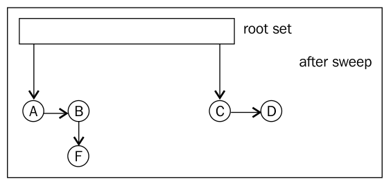
Mark and sweep
The mark and sweep algorithm is the basis of all the garbage collectors in all commercial JVMs today. Mark and sweep can be done with or without copying or moving objects. However, the real challenge is turning it into an efficient and highly scalable algorithm for memory management. The following pseudocode describes a naive mark and sweep algorithm:
Mark:
	Add each object in the root set to a queue
		For each object X in the "queue"
			Mark X reachable
			Add all objects referenced from X to the queue
Sweep:
	For each object X on the "heap"
		If the X not marked, garbage collect it
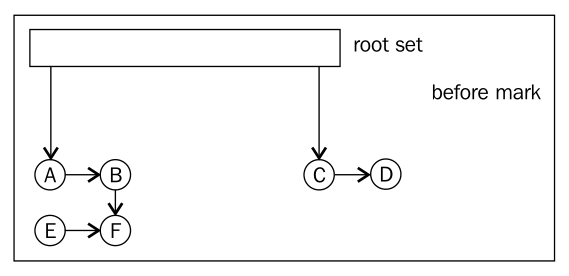
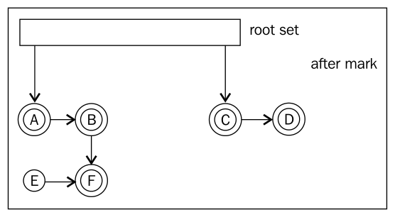
The following figures show the process of mark and sweep:
Before mark
After mark.
After sweep
In naive mark and sweep implementations, a mark bit is typically associated with each reachable object. The mark bit keeps track of if the object has been marked or not.
A variant of mark and sweep that parallelizes better is tri-coloring mark and sweep. Basically, instead of using just one binary mark bit per object, a color, or ternary value is used. There are three color: white, grey, and black.
White objects are considered dead and should be garbage collected.
Black objects are guaranteed to have no references to white objects.
Grey objects are live, but with the status of their children unknown.
Initially, there are no black object – the marking algorithm needs to find them, and the root set is colored grey to make the algorithm explore the entire reachable object graph. All other objects start out as white.
The tri-color algorithm is fairly simple:
Mark:
	All objects are White by default.
	Color all objects in the root set Grey.
	While there exist Grey objects
		For all Grey object, X
			For all white objects (successors) Y, that X references Color Y Grey.
			If all edges from X lead to another Grey object, Color X Black.
Sweep:
	Garbage collect all White objects
The main idea here is that as long as the invariant that no block nodes ever point to white nodes is maintained, the garbage collector can continue marking even while changes to the object graph take place.
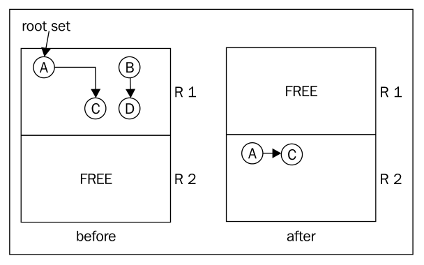
Stop and Copy
Stop and copy can be seen as a special case of tracing GC, and is intelligent in its way, but is impractical for large heap sizes in real applications.
Stop and copy garbage collection partitioning the heap into two region of equal size. Only one region is in use at a time. Stop and copy garbage collection goes through all live objects in one of the heap regions, starting at the root set, following the root set pointers to other objects and so on. The marked live objects are moved to the other heap region. After garbage collection, the heap regions are switched so that other half of the heap becomes the active region before the next collection cycle.
Advantages of stop and copy algorithm:
fragmentation can’t become an issue.
Disadvantages of stop and copy algorithm:
All live objects must be copied each time a garbage collection is performed, introducing a serious overhead in GC time as a function of the amount of live data.
Only using half of heap at a time is a waste of memory.
The following figure shows the process of stop and copy:
Generational garbage collection
In object-oriented languages, most objects are temporary or short-lived. However, performance improvement for handling short-lived objects on the heap can be had if the heap is split into two or more parts called generations.
In generational garbage collection, new objects are allocated in “young” generations of the heap, that typically are orders of magnitude smaller than the “old” generation, the main part of the heap. Garbage collection is then split into young and old collections, a young collection merely sweeping the young spaces of the heap, removing dead objects and promoting surviving objects by moving them to an older generation.
Collecting a smaller young space is orders of magnitude faster than collecting the larger old space. Even though young collections need to happen far more frequently, this is more efficient because many objects die young and never need to be promoted. ideally, total throughput is increased and some potential fragmentation is removed.
JRockit refer to the young generations as nurseries.
Muti generation nurseries
While generational GCs typically default to using just one nursery, sometimes it can be a good idea to keep several small nursery partitions in the heap and gradually age young objects, moving them from the “younger” nurseries to the “older” ones before finally promoting them to the “old” part of heap. This stands in contrast with the normal case that usually involves just one nursery and one old space.
Multi generation nurseries may be more useful in situations where heavy object allocation takes place.
If young generation objects live just a bit longer, typically if they survive a first nursery collection, the standard behavior of a single generation nursery collector, would cause these objects to be promoted to the old space. There, they will contribute more to fragmentation when they are garbage collected. So it might make sense to have several young generations on the heap, with different age spans for young objects in different nurseries, to try to keep the heap holes away from the old space where they do the most damage.
Of course the benefits of a multi-generational nursery must be balanced against the overhead of copying objects multiple times.
Write barriers
In generational GC, objects may reference other objects located in different generations of the heap. For example, objects in the old space may point to objects in the young spaces and vice versa. If we had to handle updates to all references from the old space to the young space on GC by traversing the entire old space, no performance would be gained from the generational approach. As the whole point of generational garbage collection is only to have to go over a small heap segment, further assistance from the code generator is required.
In generational GC, most JVMs use a mechanism called write barriers to keep track of which parts of the heap need to be traversed. Every time an object A starts to reference another object B, by means of B being placed in one of A’s fields or arrays, write barriers are needed.
The traditional approach to implementing write barriers is to divide the heap into a number of small consecutive sections (typically about 512 bytes each) that are called cards. The address space of the heap is thus mapped to a more coarse grained card table. whenever the Java program writes to a field in an object, the card on the heap where the object resides is “dirtied” by having the write barrier code set a dirty bit.
Using the write barriers, the traversal time problem for references from the old generation to the nursery is shortened. When doing a nursery collection, the GC only has to check the portions of the old space represented by dirty cards.
Throughput versus low latency
Garbage collection requires stopping the world, halting all program execution, at some stage. Performing GC and executing Java code concurrently requires a lot more bookkeeping and thus, the total time spent in GC will be longer. If we only care about throughput, stopping the world isn’t an issue–just halt everything and use all CUPs to garbage collect. However, to most applications, latency is the main problem, and latency is caused by not spending every available cycle executing Java code.
Thus, the tradeoff in memory management is between maximizing throughput and maintaining low latencies. But, we can’t expect to have both.
Garbage collection in JRockit
The backbone of the GC algorithm used in JRockit is based on the tri-coloring mark and sweep algorithm. For nursery collections, heavily modified variants of stop and copy are used.
Garbage collection in JRockit can work with or without generations, depending on what we are optimizing for.
Summary
First, we need to know what is automatic memory management, its advantages and disadvantages.
Fundamentals of heap management are: how to allocating and releasing objects on the heap, how to compact fragmentations of heap memory.
There are two common garbage collection algorithms: reference counting and tracing garbage collection. The reference counting is simple, but have some serious drawbacks. There are many variations of tracing techniques: “mark and sweep” and “stop and copy”. The “stop and copy” technique has some drawbacks, and it only uses in some special scenarios. Therefore, the mark and sweep is the most popular garbage collection algorithm use in JVMs.
The real-world garbage collector implementation is called generational garbage collection that is based on the “mark and sweep” algorithm.
References
[1] Oracle JRockit: The Definitive Guide by Marcus Hirt, Marcus Lagergren
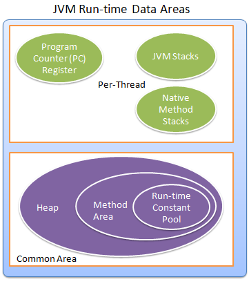
The Java Virtual Machine defines various run-time data areas that are used during execution of a program. Some of these data areas are created on Java Virtual Machine start-up and are destroyed only when the Java Virtual Machine exits. Other data areas are per thread. Per-thread data areas are created when a thread is created and destroyed when the thread exits. The data areas of JVM are logical memory spaces, and they may be not contiguous physical memory space. The following image shows the JVM run-time data areas:
The pc Register
The Java Virtual Machine can support many threads of execution at once. Each JVM thread has its own pc (program counter) register. At any point, each JVM thread is executing the code of a single method, namely the current method for that thread. If that method is not native, the pc register contains the address of the JVM instruction currently being executed. If the method is native, the value of the pc register is undefined.
Java Virtual Machine Stacks
Each JVM thread has a private JVM stack, created at the same time as the thread. A JVM stack stores frames. The JVM stack holds local variables and partial results, and plays a part in method invocation and return.
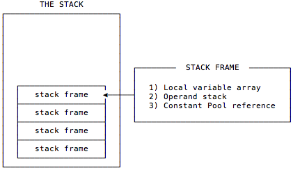
Each frame in a stack stores the current method’s local variable array, operand stack, and constant pool reference. A JVM stack may have many frames because until any method of a thread is finished it may call many other methods, and frames of these methods also store in the same JVM stack.
Because the JVM stack is never manipulated directly except to push and pop frames, frames may be heap allocated. The memory for a JVM stack does not need to be contiguous.
Frames
A frame is used to store data and partial results, as well as to perform dynamic link, return values for method, and dispatch exceptions.
A new frame is created each time a method is invoked. A frame is destroyed when its method invocation completes, whether that completion is normal or abrupt. Frames are allocated from the JVM stack of the thread creating the frame. Each frame has its own array of local variables, operand stack, and a reference to the run-time constant pool of the class of the current method.
Only one frame for the executing method, is active at any point in a given thread of control. This frame is referred to as the current frame, and its method is known as the current method. The class in which the current method is defined is the current class. Operations on local variables and the operand stack are typically with reference to the current frame.
A frame ceases to be current if its method invokes another method or if its method completes. When a method is invoked, a new frame is created and becomes current when control transfers to the new method. On method return, the current frame passes back the result of its method invocation, to the previous frame.
A frame created by a thread is local to that thread and connot be referenced by any other thread.
Heap
The JVM has a heap that is shared among all JVM threads. The heap is the run-time data area from which memory for all class instances and arrays is allocated.
The heap is created on virtual machine start-up. Heap storage for objects is reclaimed by an automatic storage management system (known as a garbage collector); objects are never explicitly deallocated. The JVM assumes no particular type of automatic storage management system, and the storage management technique may be chosen according to the implementor’s system requirements. The memory for the heap does not need to be contiguous.
Method Area
The JVM has a method area that is shared among all JVM threads. The method area is analogous to the storage area for compiled code of conventional language or analogous to the “text” segment in an operating system process. It stores per-class structures such as the run-time constant poll, field and method data, and the code for methods and constructors, including the special methods used in class and instance initialization and interface initialization.
The Method area is created on virtual machine start-up. Although the method area is logically part of the heap, simple implementations may choose not to either garbage collect or compact it. The method area may be of a fixed size or may be expanded as required. The memory for the method area does not need to be contiguous.
Run-Time Constant Pool
A run-time constant pool is a per-class or per-interface run-time representation of the constant_pool table in a class file. It contains several kinds of constant, ranging from numeric literals known at compile-time to method and field references that must be resolved at run-time. The run-time constant pool serves a function similar to that of a symbol table for a conventional programming language, although it contains a wider range of data than a typical symbol table.
Each run-time constant pool is allocated from the JVM’s method area. The run-time constant pool for a class or interface is constructed when the class or interface is created by the JVM.
References constant pools
A symbolic reference to a class or interface is in CONSTANT_Class_info structure.
A symbolic reference to a field of a class are in CONSTANT_Fieldref_info structure.
A symbolic reference to a method of a class is derived from a CONSTANT_Methodref_info structure.
A symbolic reference to a method of an interface is derived from a CONSTANT_InterfaceMethodref_info structure.
Literals constant pools
A string literal is in CONSTANT_String_info structure
Constant values are in CONSTANT_Integer_info, CONSTANT_Float_info, CONSTANT_Long_info, or CONSTANT_Double_info structures.
Native Method Stacks
JVM may use native method stacks to support native methods. The native methods are written in a language other than the Java programming language. JVM implementations that cannot load native methods and that do not themselves rely on conventional stacks need not supply native method stack. If supplied, native method stacks are typical allocated per thread when each thread is created.
How does A Program’s Running Represent in JVM Memory Area
Program start with the main method.
Before execute the main(). 1) JVM creates a thread and allocates pc register, JVM stack, native method stack run-time memory area for the main thread. 2) JVM loading the class of main() and initializes the class static resources (that stored in constant pool). 3) create a new frame for main() method and construct the frame’s structure. 4) update the pc register to refer to the first line of main().
JVM executing pc register referred instruction of the main thread.
When we need to create an instance of a class in the main() method. 1) JVM loads the calling class, and initializes its static resources 2) JVM creates a new object in heap, and initializes its members, and constructs the object.
When we calling a method of the new created object in the main(). 1) The JVM create a new frame in JVM stack for the calling method of that object, and that frame becomes current frame. 2) update pc register to refer to that method. 3) JVM executing pc register referred instruction.
Conclusion
Per-Thread Data Areas
The pc Register. It contains the address of the JVM instruction currently being executed.
Java Virtual Machine Stacks. It holds local variables and partial results.
Native Method Stacks. To support native methods.
Threads-Shared Data Areas
Heap. It contains all class instances and arrays.
Method Area. It’s part of heap. It stores per-class structures such as run-time constant poll, field and method data, and the code for methods and constructors.
Run-Time Constant Pool. It’s part of method area. It contains several kinds of constant, literals and reference constant.
写完了之后,就购买了域名和云服务器,然后就部署上去了。但是,我发现网站会偶尔访问不了,无响应。发现是服务器的程序进程挂掉了,于是重新启动项目后,我在服务器的控制面板观察服务器的资源状态,看到系统占用内存会不断的升高,所以,我猜应该是内存不足导致进程挂掉了,可是不知道为什么会导致内存泄漏。由于当时已经在网上推广了自己的网站,事情比较紧急,想着用什么方法来解决呢?于是我先是把应用程序作为 Linux 自启的系统服务,这样程序挂掉之后会自动重新启动,不至于一直访问不了。然后,我又通过加一台服务器使用 Nginx 进行负载均衡。因为程序挂掉是需要经过一段时间的,然后需要十几秒的时间重启,在相同的十几秒时间,两台服务器同时挂掉的机率比较小,通过负载均衡可以错开这十几秒,从而使得网站可以持续访问。
通过上面的 GC 日志,可以看出 HotSpot VM 把我电脑的所有可用空间(4G 多)作为了最大的堆内存空间,然后进行了若干次的 Minor GC。然后进行了一次 Full GC,增加了 Metadata 即 Permanent generation 区域的内存空间大小。然后又进行了几次 Minor GC。以上是全部的 GC 日志,后面就没有任何日志了。
通过上面的 GC 日志,可用看出 HotSpot VM 实际分配的各个区域的内存比我们设置的要稍微大一点。然后 JVM 进行了多次的 Minor GC,不断地收集 Young generation 的空间,可能 Young generation 空间设置的小了一点,但也感觉不是小了,因为只有项目刚启动时有 Minor GC,后面一直都没有 Minor GC 了。
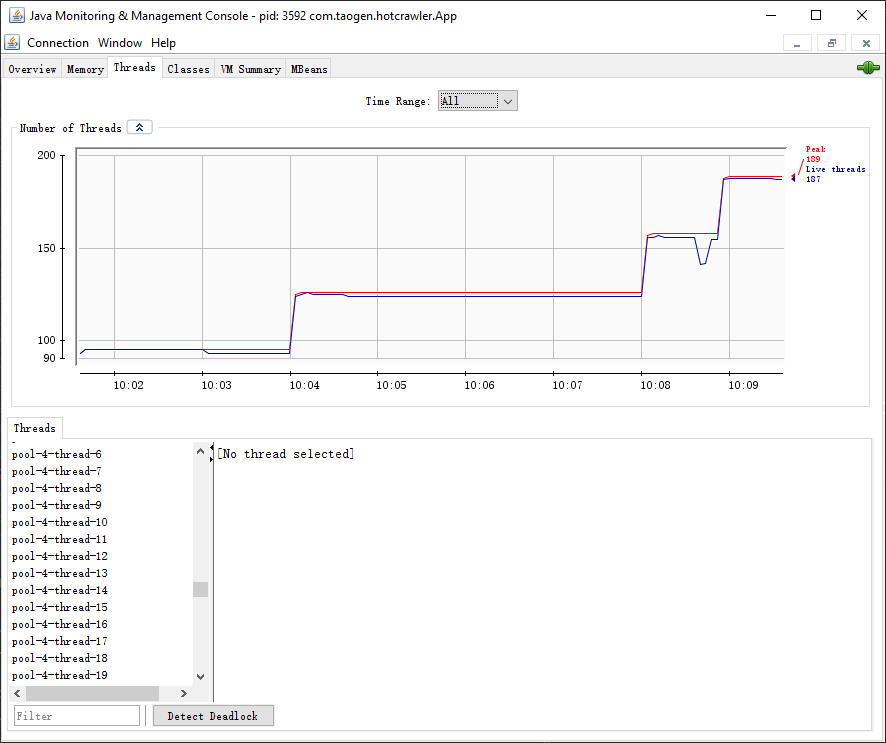
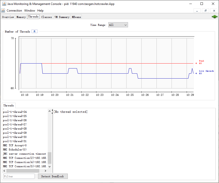
然而,重点来了,重点是现在没有了 Full GC,这说明 heap 的 Old generation 和 permanent generation 的内存是够用的。通过 Windows 操作系统的进程管理器会发现程序所占的内存远远超过 JVM 堆的内存,而且程序占用的内存还在不断的上升。通过 GC 日志感觉堆内存没什么问题,那么问题出在哪里呢?
The Proxy is a design pattern in software design. It provides a surrogate or placeholder for another object to control access to it. It lets you call a method of a proxy object the same as calling a method of a POJO. But the proxy’s methods can do additional things than POJO’s method.
Why Do We Need Proxy
It lets you control to access an object. For example, to delay an object’s construction and initialization.
It lets you track the object access. For example, tracking methods access that can analyze user behavior or analyze system performance.
How to Use Proxy in Java
There are commonly three ways to implement the proxy pattern in Java: static proxy, JDK dynamic proxy, and CGLib dynamic proxy.
Static Proxy
The static proxy implemented by reference the common class in proxy class. The following example is a basic static proxy implementation:
publicinterfaceSubject{ voidrequest(); }
publicclassRealSubjectimplementsSubject{ publicvoidrequest(){ System.out.println("request to RealSubject..."); } }
The JDK dynamic proxy implemented in package java.lang.reflect of Java API. Its underlying implementation is the Java reflection.
The manly class for implemented dynamic proxy are: the interface java.lang.reflect.InvocationHandler, and the class java.lang.reflect.Proxy.
You can call the Proxy‘s a static method Object newProxyInstance(ClassLoader loader, Class<?>[] interfaces, InvocationHandler h) to get a proxy object.
The ClassLoader instance commonly use ClassLoader.getSystemClassLoader().
The array of Class Class<?>[] is the interfaces you want to implement.
The InvocationHandler instance is an invocation handler that handling proxy method calling with the method invoke(Object proxy, Method method, Object[] args). We need to create an invocation handler by implementing the interface InvocationHandler.
The following code example is a basic JDK Dynamic proxy implementation:
publicinterfaceSubject{ voidrequest(); }
publicclassRealSubjectimplementsSubject{ publicvoidrequest(){ System.out.println("request to RealSubject..."); } }
All proxy classes extend the class java.lang.reflect.Proxy.
A proxy class has only one instance field–the invocation handler, which is defined in the Proxy superclass.
Any additional data required to carry out the proxy objects’ tasks must be stored in the invocation handler. The invocation handler wrapped the actual objects.
The name of proxy classes are not defined. The Proxy class in Java virtual machine generates class names that begin with string $Proxy.
There is only one proxy class for a particular class loader and ordered set of interfaces. If you call the newProxyInstance method twice with the same class loader and interface array, you get two objects of the same class. You can get class by Proxy.getProxyClass(). You can test whether a particular Class object represents a proxy class by calling the isProxyClass method of the Proxy class.
CGLib Dynamic Proxy
CGLib (Code Generation Library) is an open source library that capable creating and loading class files in memory during Java runtime. To do that it uses Java bytecode generation library ‘asm’, which is a very low-level bytecode creation tool. CGLib can proxy to objects without Interface.
To create a proxy object using CGLib is almost as simple as using the JDK reflection proxy API. The following code example is a basic CGLib Dynamic proxy implementation:
publicinterfaceSubject{ voidrequest(); }
publicclassRealSubjectimplementsSubject{ publicvoidrequest(){ System.out.println("request to RealSubject..."); } }
The difference between JDK dynamic proxy and CGLib is that name of the classes are a bit different and CGLib do not have an interface.
It is also important that the proxy class extends the original class and thus when the proxy object is created it invokes the constructor of the original class.
Conclusion
Differences between JDK proxy and CGLib:
JDK Dynamic proxy can only proxy by interface (so your target class needs to implement an interface, which is then also implemented by the proxy class). CGLib (and javassist) can create a proxy by subclassing. In this scenario the proxy becomes a subclass of the target class. No need for interfaces.
JDK Dynamic proxy generates dynamically at runtime using JDK Reflection API. CGLib is built on top of ASM, this is mainly used the generate proxy extending bean and adds bean behavior in the proxy methods.
References
[1] Core Java Volume I Fundamentals by S, Horstmann
[2] Design Patterns: Elements of Reusable Object-Oriented Software by Erich Gamma, Richard Helm, Ralph Johnson, John Vlissides
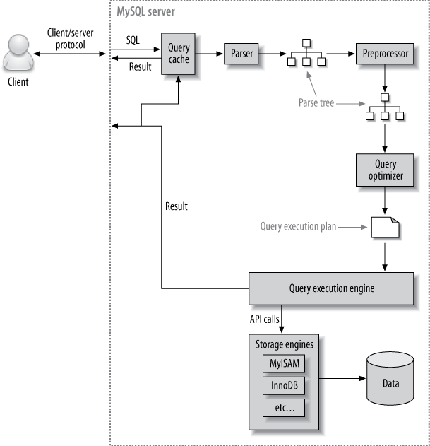
The EXPLAIN command is the main way to find out how the query optimizer decides to execute queries. This feature has limitations and doesn’t always tell the truth, but its output is the best information available. Interpreting EXPLAIN will also help you learn how MySQL’s optimizer works.
Invoking EXPLAIN
To use EXPLAIN, simply add the word EXPLAIN just before the SELECT keyword in your query. MySQL will set a flag on the query. When it executes the query, the flag cases it to return information about each step in the execution plan, instead of executing it. It returns one or more rows, which show each part of the execution plan and the order of execution. There is a simple example of EXPLAIN query statement:
EXPLAIN SELECT1;
There is one row in the output per table in the query. If the query joins two tables, there will be two rows of output. The meaning of “table” is fairly broad meaning: it can mean a subquery, a UNION result, and so on.
It’s a common mistake that MySQL doesn’t execute a query when you add EXPLAIN to it. In fact, if the query contains a subquery in the FROM clause, MySQL actually executes the subquery, places its results into a temporary table, and finishes optimizing the outer query. It has to process all such subqueries before it can optimize the outer query fully, which it must do for EXPLAIN. This means EXPLAIN can actually cause a great deal of work for the server if the statement contains expensive subqueries or views that use the TEMPTABLE algorithm.
EXPLAIN is an approximation. Sometimes it’s a good approximation, but at other times, it can be very far from the truth. Here are some of its limitation:
EXPLAIN doesn’t tell you anything about how triggers, stored functions, or UDFs will affect your query.
It doesn’t work for stored procedures.
It doesn’t tell you about optimization MySQL does during query execution.
Some of the statistics it shows are estimates and can be very inaccurate.
It doesn’t show you everything there is to know about a query’s execution plan.
It doesn’t distinguish between some things with the same name. For example, it uses “filesort” for in-memory sorts and for temporary files, and it displays “Using temporary” for temporary tables on disk and in memory.
Rewriting Non-SELECT Queries
MySQL explain only SELECT queries, not stored routine calls or INSERT, UPDATE, DELETE, or any other statements. However, you can rewrite some non-SELECT queries to be EXPLAIN-able. To do this, you just need to convert the statement into an equivalent SELECT that accesses all the same columns. Any columns mentioned must be in a SELECT list, a join clause, or a WHERE clause. Note that since MySQL 5.6, it can explain INSERT, UPDATE, and DELETE statements.
For example:
UPDATE actor INNERJOIN film_actor USING(actor_id) SET actor.last_update=film_actor.last_update;
To
EXPLAIN SELECT actor.last_update, film_actor.last_update FROM actor INNERJOIN film_actor USING(actor_id)
The Columns in EXPLAIN
EXPLAIN’s output always has the same columns, which adds a filtered column in MySQL 5.1.
Keep in mind that the rows in the output come in the order in which MySQL actually executes the parts of the query, which is not always the same as the order in which they appear in the original SQL. In EXPLAIN of MySQL, there are columns: id, select_type, table, partitions, type, possible_keys, key_len, ref, rows, filtered, Extra.
The id Column
The column always contains a number, which identifies the SELECT to which the row belongs.
MySQL divides SELECT queries into simple and complex types, and the complex types can be grouped into three broad classes: simple subqueries, derived tables (subqueries in the FROM clause), and UNIONs. Here is a simple subquery example:
EXPLAIN SELECT (SELECT1FROM sakila.actor LIMIT 1) FROM sakila.film;
+----+-------------+-------+...
| id | select_type | table |...
+----+-------------+-------+...
| 1  | PRIMARY     | film  |...
| 2  | SUBQUERY    | actor |...
+----+-------------+-------+...
Here is a derived tables query example:
EXPLAIN SELECT film_id FROM (SELECT film_id FROM sakila.film) AS der;
+------+--------------+------------+...
| id   | select_type  | table      |...
+------+--------------+------------+...
| 1    | PRIMARY      | NULL       |...
| 2    | UNION        | NULL       |...
| NULL | UNION RESULT | <union1,2> |...
+------+--------------+------------+...
UNION results are always placed into an anonymous temporary table, and MySQL then reads the results back out of the temporary table. The temporary table doesn’t appear in the original SQL, so its id columns is NULL.
The select_type Column
This column shows whether the row is a simple or complex SELECT (and if it’s the latter, which of the three complex types it is). The value SIMPLE means the query contains no subqueries or UNIONs. If the query has any such complex subparts, the outermost part is labeled PRIMARY, and other parts are labeled as follows:
SUBQUERY. A SELECT that is contained in a subquery in the SELECT clause (not in the FROM clause) is labeled SUBQUERY.
DERIVED. A SELECT that is contained in a subquery in the FROM clause. The server refers to this as a “derived table” internally, because the temporary table is derived from the subquery.
UNION. The second and subsequent SELECTs in a UNION are labeled as UNION. The first SELECT is labeled PRIMARY as though it is executed as part of the outer query.
UNION RESULT. The SELECT used to retrieve results from the UNION’s anonymous temporary table is labeled as UNION RESULT.
In addition to these values, a SUBQUERY and a UNION can be labeled as DEPENDENT and UNCACHEABLE. DEPENDENT means the SELECT depends on data that is found in an outer query; UNCACHEABLE means something in the SELECT prevents the result form being cached with an Item_cache (such as the RAND() function).
UNCACHEABLE UNION example:
EXPLAIN select tmp.id FROM (SELECT*FROM test t1 WHERE t1.id=RAND() UNIONALL SELECT*FROM test t2 WHERE t2.id=RAND()) AS tmp;
This column shows which table the row is accessing. It’s the table, or its alias. The number of the rows in EXPLAIN equals the sum of number of SELECT, JOIN and UNION.
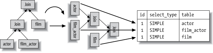
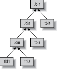
MySQL’s query execution plans are always left-deep trees. The leaf nodes in order correspond directly to the rows in EXPLAIN. For example:
The table column becomes much more complicated when there is a subquery in the FROM clause or a UNION. In these cases, there really isn’t a “table” to refer to, because the anonymous temporary table MySQL creates exists only while the query is executing.
When there’s a subquery in the FROM clause, the table column is of the form <derivedN>, where N is the subquery’s id. This always a “forward reference”. In other words, N refers to a later row in the EXPLAIN output.
When there’s a UNON, the UNION RESULT table column contains a list of ids that participate in the UNION. This is always a “backward reference”, because the UNION RESULT comes after all of the rows that participate in the UNION.
+------+----------------------+------------+...
| id   | select_type          | table      |...
+------+----------------------+------------+...
| 1    | PRIMARY              | <derived3> |...
| 3    | DERIVED              | actor      |...
| 2    | DEPENDENT SUBQUERY   | film_actor |...
| 4    | UNION                | <derived6> |...
| 6    | DERIVED              | film       |...
| 7    | SUBQUERY             | store      |...
| 5    | UNCACHEABLE SUBQUERY | rental     |...
| NULL | UNION RESULT         | <union1,4> |...
+------+----------------------+------------+...
Reading EXPLAIN’s output often requires you to jump forward and backward in the list.
The type Column
The MySQL manual says this column shows the “join type”, but it’s more accurate to say the access type. In other words, how MySQL has decided to find rows in the table. Here are the most important access methods, from worst to best:
ALL. This means a table scan. MySQL must scan through the table from beginning to end to find the row. (There are exceptions, such as queries with LIMIT or queries that display “Using distinct/not exist” in the Extra column.)
index. This means an index scan. The main advantage is that this avoids sorting. The biggest disadvantage is the cost of reading an entire table in index order. This usually means accessing the rows in random order, which is very expensive. If you also see “Using index” in the Extra column, it means MySQL is using a covering index. This is much less expensive than scanning the table in index order.
range. A range scan is a limited index scan. It begins at some point in the index and returns rows that match a range of values. This is better than a full index scan because it doesn’t go through the entire index. Obvious range scans are queries with a BETWEEN or > in the WHERE clause.
ref. This is an index access (or index lookup) that returns rows that match a single value. The ref_or_null access type is a variation on ref. It means MySQL must do a second lookup to find NULL entries after doing the initial lookup.
eq_ref. This is an index lookup that MySQL knows will return at most a single value. You will see this access method when MySQL decides to use a primary key or unique index to satisfy the query by comparing it to some reference value.
const, system. MySQL uses these access types when it can optimize away some part of the query and turn it into a constant. The table has at most one matching row, which is read at the start of the query. For example, if you select a row’s primary key by placing it primary key into then where clause. e.g SELECT * FROM <table_name> WHERE <primary_key_column>=1;
NULL. This access method means MySQL can resolve the query during the optimization phase and will not even access the table or index during the execution stage. For example, selecting the minimum value from an indexed column can be done by looking at the index alone and requires no table access during execution.
Other types
fulltext. The join is performed using a FULLTEXT index.
index_merge. This join type indicates that the Index Merge optimization is used. In this case, the key column in the output row contains a list of indexes used. Indicates a query to make limited use of multiple indexes from a single table. For example, the film_actor table has an index on film_id and an index on actor_id, the query is SELECT film_id, actor_id FROM sakila.film_actor WHERE actor_id = 1 OR film_id = 1
unique_subquery. This type replaces eq_ref for some IN subqueries of the following form. value IN (SELECT primary_key FROM single_table WHERE some_expr)
index_subquery. This join type is similar to unique_subquery. It replaces IN subqueries, but it works for nonunique indexes in subqueries. value IN (SELECT key_column FROM single_table WHERE some_expr)
The possible_keys Column
This column shows which indexes could be used for the query, based on the columns the query accesses and the comparison operators used. This list is created early in the optimization phase, so some of the indexes listed might be useless for the query after subsequent optimization phases.
The key Column
This column shows which index MySQL decided to use to optimize the access to the table. If the index doesn’t appear in possible_keys, MySQL chose it for another reason–for example, it might choose a covering index even when there is no WHERE clause.
In other words, possible_keys reveals which indexes can help make row lookups efficient, but key shows which index the optimizer decided to use to minimize query cost.
Here’s an example:
EXPLAIN SELECT actor_id, film_id FROM sakila.film_actor;
*************************** 1. row ***************************
id: 1
select_type: SIMPLE
table: film_actor
type: index
possible_keys: NULL
key: idx_fk_film_id
key_len: 2
ref: NULL
rows: 5143
Extra: Using index
The key_len Column
This column shows the number of bytes MySQL will use in the index. If MySQL is using only some of the index’s columns, you can use this value to calculate which columns it uses. Remember that MySQL 5.5 and older versions can use only the left most prefix of the index. For example, file_actor’s primary key covers two SMALLINT columns, and a SMALLINT is two bytes, so each tuple in the index is four bytes. Here’s a query example:
EXPLAIN SELECT actor_id, film_id FROM sakila.film_actor WHERE actor_id=4;
You can use EXPLAIN to get how many bytes in one row of the index, then to calculate the query uses how much rows index by the key_len of the EXPLAIN.
MySQL doesn’t always show you how much of an index is really being used. For example, if you perform a LIKE query with a prefix pattern match, it will show that the full width of the column is being used.
The key_len column shows the maximum possible length of the indexed fields, not the actual number of bytes the data in the table used.
The ref Column
This column shows which columns or constant from preceding tables are being used to look up values in the index named in the key column.
The rows Column
This column shows the number of rows MySQL estimates it will need to read to find the desired rows.
Remember, this is the number of rows MySQL thinks it will examine, not the number of rows in the result set. Also realize that there are many optimizations, such as join buffers and caches, that aren’t factored into the number of rows shown.
The filtered Column
This column shows a pessimistic estimate of the percentage of rows that will satisfy some condition on the table, such as a WHERE clause or a join condition. If you multiply the rows column by this percentage, you will see the number of rows MySQL estimates it will join with the previous tables in the query plan.
The Extra Colum
This column contains extra information that doesn’t fit into other columns. The most important values you might frequently are as follows:
Using index. This indicates that MySQL will use a covering index to avoid accessing the table.
Using where. This means the MySQL server will post-filter rows after the storage engine retrieves them.
Using temporary. This means MySQL will use a temporary table while sorting the query’s result.
Using filesort. This means MySQL will use an external sort to order the results, instead of reading the rows from the table in index order. MySQL has two filesort algorithms. Either type can be done in memory or on disk. EXPLAIN doesn’t tell you which type of filesort MySQL will use, and it doesn’t tell you whether the sort will be done in memory or on disk.
Range checked for each record (index map:N). This value means there’s no good index, and the indexes will be reevaluated for each row in a join. N is a bitmap of the indexes shown in possible_keys and is redundant.
Using index condition: Tables are read by accessing index tuples and testing them first to determine whether to read full table rows.
Improvements in MySQL 5.6
Some EXPLAIN improvements in MySQL 5.6
To explain queries such as UPDATE, INSERT, and so on.
A variety of improvements to the query optimizer and execution engine that allow anonymous temporary tables to be materialized as late as possible, rather than always creating and filling them before optimizing and executing the portions of the query that refer to them. This will allow MySQL to explain queries with subqueries instantly, without having to actually execute the subqueries first.
Conclusion
The most important columns of EXPLAIN are type and Extra. They determine does the query uses an index or covering index.
the most important access methods (the type column of EXPLAIN), from worst to best:
ALL
index
range
ref
eq_ref
const, system
NULL
References
[1] High Performance MySQL by Baron Schwartz, Vadim Tkachenko, Peter Zaitsev, Derek J. Balling
Using general principles and best practices to create your table schema.
Understanding the structure and properties of different kinds of indexes, and to choose a proper kind of index.
According to query statements in your application to create indexes, creates as few indexes as possible. And makes your indexes covering as more frequently selected columns as possible.
Using EXPLAIN to check how a query execution.
Using query profiling to determine which strategy is optimal, or which query is faster.
Common Strategies for MySQL Optimization
Schema
Choosing optimal data types.
Denormalization.
Cache and Summary Tables.
Index
Common indexes such as B-Tree, Hash, and Bitmap.
Multi-column indexes and covering indexes, prefix indexes and compressed indexes.
Avoid to add redundant and duplicate indexes, and remove unused indexes.
Query
Queries tricks. For example, chopping up a query (or finding difference set).
Join decomposition. Converting join to single-table queries.
Using query optimizer hints.
Optimizing specific types of queries.
Do complex operations in application programs instead of in database systems. Complex operations: join, nested subqueries, group by, order by.
This post is talking about MySQL query optimization, if you are familiar with this topic, you can go to the conclusion part that’s a good summary of the query optimization in MySQL that may give you some enlightenment.
Schema optimization and indexing, which are necessary for high performance. But they are not enough, you also need to design your queries well. If your queries are bad, even the best-designed schema and indexes will not perform well.
We need to understand deeply how MySQL really executes queries, so you can reason about what is efficient or inefficient, exploit MySQL’s strengths, and avoid its weakness.
Why Are Queries Slow
Before trying to write fast queries, you need to know the good or bad queries are determined by response time. Queries are tasks, but they are composed of subtasks, and those subtasks consume time. To optimize a query, you must optimize its subtasks by eliminating them, make them happen fewer times, or making them happen more quickly.
You can use profiling a query to find out what subtasks performs to execute a query, and which ones are slow. In general, you can think of a query’s lifetime by following the query through its sequence from the client to the server, where it is parsed, planned, and executed, and then back again to the client. Execution is one of the most important stages in a query’s lifetime. It involves lots of calls to the storage engine to retrieve rows, as well as post-retrieval operations such as grouping and sorting.
While accomplishing all these tasks, the query spends time on the network, in the CPU, in operations (such as statistics and planning, locking, and call the storage engine to retrieve rows).
In every case, excessive time may be consumed because the operations are performed needless, performed too many times, or are too slow. The goal of optimization is to avoid that, by eliminating or reducing operations, or making them faster. For do this optimization, we need to understanding a query’s lifecycle and thinking in terms of where the time is consumed.
Slow Query Basic: Optimize Data Access
The most basic reason a query doesn’t perform well is because it’s working with too much data. We can use the following methods to find out whether your query is access to more data than it needs.
Find out whether your application is retrieving more data than you need. That means it’s accessing too many rows, or accessing too many columns.
Find out whether the MySQL server is analyzing more rows than it needs.
Are You Asking the Database for Data You Don’t Need
Some query ask for more data than they need and then throw some of it away. This demands extra work of the MySQL server, adds network overhead, and consumes memory and CPU resources on the application server.
The common mistakes of fetching more data
Fetching more rows than needed.
Fetching all columns from a multi-table join.
Fetching all columns.
Fetching the same data repeatedly. You don’t need to fetch multiple times for the same data. You could cache it the first time you fetch it, and reuse it thereafter.
Is MySQL Examining Too Much Data
Once you are sure your queries retrieve only the data you need, you can look for queries that examine too much data while generating results. In MySQL, the simplest query cost metrics are:
Response time.
Number of rows examined
Number of rows returned
None of these metrics is a perfect way to measure query cost, but they reflect roughly how much data access to execute a query and translate approximately into how fast the query runs. All three metrics are logged in the query log, so looking at the query log is one of the best ways to find queries that examine too much data.
Response time
Response time is the sum of two things: service time and queue time. Service time is how long it takes the server to actually process the query. Queue time is the portion of response time during which the server isn’t really executing the query–it’s waiting for something, such as I/O, row lock and so forth. As a result, response time is not consistent under varying load conditions. When you look at a query’s response time, you should ask yourself whether the response time is reasonable for the query.
Rows examined and rows return
It’s useful to think about the number of rows examined when analyzing queries, because you can see how efficiently the queries are finding data you need.
However, not all row accesses are equal. Shorter rows are faster to access, and fetching rows form memory is much faster than reading them from disk.
Ideally, the number of rows examined would be the same as the number returned, but in practice this rarely possible. For example, when constructing rows with joins.
Rows examined and access types
MySQL can use several access methods to find and return a row. Some require examining many rows, but others might be without examining any.
The access methods appear in the type column in EXPLAIN’s output. The access types range from a full table scan to index scans, range scans, unique index lookups, and constants. Each of these is faster than the one before it, because it requires reading less data.
If you aren’t getting a good access type, the best way to solve the problem is usually by adding an appropriate index.
In general, MySQL can apply a WHERE clause in three ways, from best to worst:
Apply the conditions to the index lookup operation to eliminate nonmatching rows. This happen at the storage engine layer.
Use a covering index (“Using index” in the Extra column of EXPLAIN) to avoid row accesses and filter out nonmatching rows after retrieving each result from the index.
Retrieve rows from the table, then filter nonmatching rows (“Using where” in the Extra column of EXPLAIN). This happens at the server layer.
Good indexes help your queries get a good access type and examine only the rows they need. However, adding an index doesn’t always mean that MySQL will access fewer rows, or access and return the same number of rows. For example, a query that uses the COUNT() aggregate function.
If you find that a huge number of rows were examined to produce relatively few rows in the result, you can try some more sophisticated fixes:
Use covering indexes.
Change the schema.
Rewrite a complicated query.
Ways to Restructure Queries
As you optimize problematic queries, your goal should be to find alternative ways to get the result you want. You can sometimes transform queries into equivalent forms that return the same results, and get better performance.
Complex Queries Versus Many Queries
It’s a good idea to use as few queries as possible, but sometimes you can make a query more efficient by decomposing it and executing a few simple queries instead of one complex one.
Chopping Up a Query
Another way to slice up a query is to divide and conquer, keeping it essentially the same but running it in smaller “chunks” that affect fewer rows each time.
Purging old data is a great example. For example:
DELETEFROM messages WHERE created < DATE_SUB(NOW(), INTERVAL3MONTH);
It might also be a good idea to add some sleep time between the DELETE statements to spread the load over time and reduce the amount of time locks are held.
Join Decomposition
Many high-performance applications use join decomposition. You can decompose a join by running multiple single-table queries instead of a multitable join. For example:
SELECT*FROM tag JOIN tag_post ON tag_post.tag_id=tag.id JOIN post ON tag_post.post_d=post.id WHERE tag.tag='mysql';
replace to
SELECT*FROM tag WHERE tag='mysql'; SELECT*FROM tag_post WHERE tag_id=1234; SELECT*FROM post WHERE post.id in (123,456,567,8876);
Advantages of multiple single-table queries
Caching can be more efficient.
Executing the queries individually can sometimes reduce lock contention.
The queries themselves can be more efficient.
You can reduce redundant row accesses.
Query Execution Basics
If you need to get high performance from your MySQL server, one of the best ways to learning how MySQL optimizes and executes queries.
The process MySQL to execute queries:
The client sends the SQL statement to the server.
The server checks the query cache. If there’s a hit, it returns the stored result from the cache, otherwise to next step.
The server parses, preprocesses, and optimizes the SQL into a query execution plan.
The query execution engine executes the plan by making calls to the storage engine API.
The server sends the result to the client.
The MySQL Client/Server Protocol
The protocol is half-duplex, which means that at any given time the MySQL server can be either sending or receiving messages, but not both. This protocol makes MySQL communication simple and fast, but it have some limitation. For example, once one side sends a message, the other side must fetch the entire message before responding.
The client sends a query to the server as a single packet of data. So max_allowed_packet configuration variable is important if you have large queries.
In contrast, the response from the server usually consist of many packets of data. When the server responds, the client has to receive the entire result set. Most libraries that connect to MySQL let you either fetch the whole result and buffer it in memory, or fetch each row as you need it.
Query States
Each MySQL connection, or thread, has a state that shows what it is doing at any given time. There are several ways to view these states, but the easiest is to use the SHOW FULL PROCESSLIST command. The basic states in MySQL:
Sleep
Query
Locked
Analyzing and statistics
Copying to tmp table [on disk]
Sorting result
Sending data
The Query Cache
Before parsing a query, MySQL checks for it in the query cache, if the cache is enabled. This operation is a case-sensitive hash lookup. If the query differs from a similar query in the cache by even a single byte, it won’t match.
If MySQL does find a match in the query cache, it must check privileges before returning the cache query. If the privileges are OK, MySQL retrieves the stored result from the query cache and sends it to the client. The query is never parsed, optimized, or executed.
The Query Optimization Process
After doesn’t find a match in the query cache, the next step in the query lifecycle turns a SQL query into an execution plan for the query execute engine. It has several substeps: parsing, preprocessing, and optimization. Errors (like syntax errors) can be raised at any point in the process.
The parser and the preprocessor
query parsing: MySQL’s parser breaks the query into tokens and builds a parse tree from them. The parser uses MySQL’s SQL grammar to interpret and validate the query.
query preprocessing: the preprocessor checks the resulting parse tree for additional semantics. For example, it checks that tables and columns exist, and it resolves names and aliases to ensure that column references aren’t ambiguous. Next, the preprocessor checks privileges.
The query optimizer
After preprocessing the parse tree is now valid and ready for the optimizer to turn it into a query execution plan. A query can often be executed many different ways and produce the same result. The optimizer’s job is to find the best option.
MySQL uses a cost-based optimizer, which means it tries to predict the cost of various execution plans and choose the least expensive. The unit of cost way originally a single random 4KB data page read, but also includes factors such as the estimated cost of executing a WHERE clause comparison. You can see how expensive the optimizer estimated a query to be by running the query, then inspecting the Last_query_cost session variable:
SELECT SQL_NO_CACHE COUNT(*) FROM your_table; SHOW STATUS LIKE'Last_query_cost';
Result of SHOW STATUS LIKE 'Last_query_cost' means that the optimizer estimated it would need to do about how much random data page reads to execute the query.
The optimizer might not always choose the best plan, for many reasons:
The statistics could be wrong.
The cost metric is not exactly equivalent to the true cost of running the query.
MySQL’s idea of optimal might not match yours. MySQL doesn’t really try to make queries fast; it tries to minimize their.
MySQL doesn’t consider other queries that are running concurrently.
MySQL doesn’t always do cost-based optimization.
The optimizer doesn’t take into account the cost of operations not under its control, such as executing stored functions.
MySQL’s join execution strategy
MySQL consider every query a join–not just every query that matches rows from two tables, but every query. It’s very important to understand how MySQL executes joins.
MySQL’s join execution strategy is simple: it treats every join as a nested-loop join. This means MySQL runs a loop to find a row from a table, then run a nested loop to find a matching row in the next table. It continues until it has found a matching row in each table in the join. For example:
SELECT tab1.col1, tab2.col2 FROM tab1 INNERJOIN tab2 USING(col3) WHERE tab1.col1 in (5, 6);
following pseudocode shows how MySQL might execute the query:
outer_iter = iterator over tbl1 where col1 IN(5,6)
outer_row = outer_iter.next
while outer_row
	inner_iter = iterator over tbl2 where col3 = outer_row.col3
	inner_row = inner_iter.next
	while inner_row
		output [ outer_row.col1, inner_row.col2 ]
		inner_row = inner_iter.next
	end
	outer_row = outer_iter.next
end
First Finding table iterator that fulfills the WHERE condition, then finding equal values on join columns.
The execution plan
MySQL doesn’t generate byte-code to execute a query, instead, the query execution plan is actually a tree of instructions that the query execution engine follows to produce the query results.
Any multitable query can conceptually be represent as a tree. MySQL always begins with one table and finds matching rows in the next table. Thus, MySQL’s query execution plans always take the form of left-deep tree. As shown in the figure below.
The join optimizer
The most important part of the MySQL query optimizer is the join optimizer, which decides the best order of execution for multitable queries.
MySQL’s join optimizer can reorder queries to make them less expensive to execute. You can use STRAIGHT_JOIN and write queries in the order you think is best, but such times are rare. In most cases, the join optimizer will outperform a human.
Sort optimizations
Sorting results can be a costly operation, so you can often improve performance by avoiding sorts or by performing them on fewer rows.
When MySQL can’t use an index to produce a sorted result, it must sort the rows itself. It can do this in memory or on disk, but it always calls this process a filesort, even if it doesn’t actually use a file.
If the values to be sorted will fit into the sort buffer, MySQL can perform the sort entirely in memory with a quiksort. If MySQL can’t do the sort in memory, it performs it on disk by sorting the values in chunks with quicksort, and then merges the sorted chunks into results.
When sorting a join, if the ORDER BY clause refers only to columns from the first table in the join order, MySQL can filesort this table and then proceed with the join. This case will show “Using filesort” in the Extra column of EXPLAIN. If ORDER BY clause contains columns from more than one table, MySQL must store the query’s results into a temporary table and then filesort then temporary table after the join finishes. This case will show “Using temporary; Using filesort” in the Extra column of EXPLAIN.
The Query Execution Engine
The parsing and optimizing stage outputs a query execution plan, which MySQL’s query execution engine uses to process the query. The plan is a data structure; it is not executable byte-code, which is how many other database execute queries.
In contrast to the optimization stage, the execution stage is usually not all that complex: MySQL simply follows the instructions given in the query execution plan. Many of the operations in the plan invoke methods implemented by the storage engine interface, also known as the handler API.
To execute the query, the server just repeats the instructions until there are no more rows to examine.
Returning Results to the Client
The final step in executing a query is to reply to the client. Even queries that don’t return a result set still reply to the client connection with information about the query, such as how many rows it affected.
The server generates and sends results incrementally. As soon as MySQL processes the last table and generates one row successfully, it can and should send that row to the client. This has two benefits: it lets the server avoid holding the row in memory, and it means the client starts getting the results as soon as possible. Each row in the result set is sent in a separate packet in the MySQL client/server protocol, although protocol packets can be buffered and sent together at the TCP protocol layer.
Limitations of the MySQL Query Optimizer
Correlated Subqueries
MySQL sometimes optimizes subqueries very badly. The worst offenders are IN() subqueries in the WHERE clause.
The standard advice for this query is to write it as a LEFT OUTER JOIN instead of using a subquery.
UNION Limitations
You should put condition clauses inside each part of the UNION.
For example, if you UNION together two tables and LIMIT the result to the first 20 rows:
Query 1:
This query will store all rows of tables into a temporary table then fetch first 20 rows form that temporary table.
(SELECT first_name, last_name FROM sakila.actor ORDERBY last_name) UNIONALL (SELECT first_name, last_name FROM sakila.customer ORDERBY last_name) LIMIT 20;
Query 2:
This query will store first 20 rows each table into a temporary table and then fetch first 20 rows from that temporary table.
You should use query 2 (contains inside LIMIT) instead of query 1 (only outer LIMIT).
SELECT and UPDATE on the Same Table
MySQL doesn’t let you SELECT from a table while simultaneously running an UPDATE on it. To work around this limitation, you can use a derived table, because MySQL materializes it as a temporary table.
UPDATE tb1 AS outer_tb1 SET cnt = ( SELECTcount(*) tb1 AS inner_tb1 WHERE inner_tb1.type = outer_tb1.type );
To
UPDATE tb1 INNERJOIN( SELECT type, count(*) as cnt FROM tb1 GOURP BY type ) AS der USING(type) SET tb1.cnt = der.cnt;
Query Optimizer Hints
MySQL has a few optimizer hints you can use to control the query plan if you are not content with the one MySQL’s optimizer chooses. You place the appropriate hint in the query whose plan you want to modify, and it is effective for only that query. Some of them are version-dependent. You can check the MySQL manual for the exact syntax of each hint.
STRAIGHT_JOIN. Putting this hint in after the SELECT keyword that forces all tables in the query to be joined in the order in which they are listed in the statement. Putting in between two joined tables that force a join order on the two tables between which the hint appears. It is useful when MySQL doesn’t choose a good join order, or when the optimizer takes a long time to decide on a join order.
select a.id, c.id
from a
straight_join b on b.a_id = a.id
join c on c.id = b.c_id
or
select straight_join a.id, c.id
from a
b on b.a_id = a.id
join c on c.id = b.c_id
USE INDEX, IGNORE INDEX, and FORCE INDEX. These hints tell the optimizer which indexes to use or ignore for finding rows in a table.
Optimizing Specific Types of Queries
There are some advice on how to optimize certain kinds of queries. Most of the advice is version-dependent, and it might not hold for future versions of MySQL.
Optimizing COUNT() Queries
Before optimization, it’s important that you understand what COUNT() really does.
The COUNT() counts how many times that expression has a value. When you want to know the number of rows in the result, you should always use COUNT(*).
Simple Optimizations
Example 1:
SELECTCOUNT(*) FROM world.City WHERE ID >5;
replace to
SELECT (SELECTCOUNT(*) FROM world.City) -COUNT(*) FROM world.City WHERE ID <=5;
Example 2:
SELECTSUM(IF(color ='blue', 1, 0)) AS blue,SUM(IF(color ='red', 1, 0)) AS red FROM items;
replace to
SELECTCOUNT(color ='blue'ORNULL) AS blue, COUNT(color ='red'ORNULL) AS red FROM items;
Using an approximation
Sometimes you don’t need an accurate count, so you can just use an approximation. The optimizer’s estimated rows in EXPLAIN often serves well for this. Just execute an EXPLAIN query instead of the real query.
EXPLAIN selectCOUNT(*) from your_table;
Fast, accurate, and simple: pick any two.
Optimizing JOIN Queries
There are some principles for optimizing JOIN queries:
Make sure there are indexes on the columns in the ON or USING clauses. Consider the join order when adding indexes. In general, you need to add indexes only on the second table in the join order (for example, table A join B, you need add index on B rather than A), unless they’re needed for some other reason.
Try to ensure that any GROUP BY or ORDER BY expression refers only to columns from a single table, so MySQL can try to use an index for that operation.
Be careful when upgrading MySQL, because the join syntax, operator precedence, and other behaviors have changed at various time.
Optimizing Subqueries
The core of the post is focused on MySQL 5.1 and MySQL 5.5. In these versions of MySQL, and in most situations, you should usually prefer a join where possible, rather than subqueries. However, prefer a join is not future-proof advice, so you need be cautious with it.
Optimizing GROUP BY and DISTINCT
MySQL optimizing these two kinds of queries similarly in many cases, and in fact converts between them as needed internally during then optimization process.
MySQL has two kinds of GROUP BY strategies when it can’t use an index: it can use a temporary table or file sort to perform the grouping. Either one can be more efficient for any given query. You can force the optimizer to choose one method or the other with the SQL_BIG_RESULT and SQL_SMALL_RESULT optimizer hints.
If you need to group a join by a value that comes from a lookup table, it is usually more efficient to group by the lookup table’s identifier than by value.
It’s generally a bad idea to select nongrouped columns in a grouped query, because the results will be nondeterministic and could easily change if you change an index or the optimizer decides to use a different strategy. It’s better to be explicit. We suggest you set the server’s SQL_MODE configuration variable to include ONLY_FULL_GROUP_BY so it produces an error instead of letting you write a bad query. Query select values only are grouped columns or aggregate function on grouped columns. For example:
SELECT name, COUNT(*) FROM your_table GROUPBY name;
MySQL automatically orders grouped queries by the columns in the GROUP BY clause, unless you specify an ORDER BY clause explicitly. If you don’t care about the order and you see this causing a filesort, you can use ORDER BY NULL to skip the automatic sort.
Optimizing GROUP BY WITH ROLLUP
A variation on grouped queries is to ask MySQL to do superaggregation within the results. You can do this with a WITH ROLLUP clause, but it might not be as well optimized as you need. Check the execution method with EXPLAIN , paying attention to whether the grouping is done via filesort or temporary table; try removing the WITH ROLLUP and seeing if you get the same group method.
Sometimes it’s more efficient to do superaggregation in your application, even if it means fetching many more rows from the server.
Optimizing LIMIT and OFFSET
Queries with LIMITs and OFFSETs are common in systems that do pagination, nearly always in conjunction with an ORDER BY clause. It’s helpful to have an index that supports the ordering; otherwise, the server has to do a lot of filesorts.
A frequent problem is having high value for offset. For example, if you query looks like LIMIT 10000, 20, it is generating 10020 rows and throwing away the first 10000 of them, which is very expensive. To optimize them, you can either limit how many pages are permitted in a pagination view, or try to make the high offsets more efficient.
The key of optimizing do pagination is using an index to sort rather than using a filesort. You can use join or using some methods to replace the OFFSET.
using index for sort
Using join. SELECT * FROM ... JOIN (SELECT id ... ORDER BY .. LIMIT off, count)
Remove offset. SELECT * ... ORDER BY ... LIMIT count
Remove offset and limit. SELECT * ... WHERE <column> BETWEEN <start> AND <end> ORDER BY ...
Using filesort
SELECT * ... ORDER BY ... LIMIT offset, row_count
Optimizing sort by using joins
One ways to optimizing the high value offset is offset on a covering index, rather than the full rows. You can then join the result to the full row and retrieve the additional columns you need. For example:
SELECT film_id, description FROM sakila.film ORDERBY title LIMIT 50, 5;
replace to
SELECT film.film_id, film.description FROM sakila.film INNERJOIN ( SELECT film_id FROM sakila.film ORDERBY title LIMIT 50, 5 ) AS lim USING(film_id);
SELECT id FROM your_table ORDER BT title can use the covering index(title, id). However, SELECT * ... ORDER BY title have no index to use because in general there is no covering all column index in a table, and it has to using filesort.
Optimizing offset by using positional range queries
Limit to a positional query, which the server can executes as an index range scan. For example:
SELECT film_id, description FROM sakila.film WHERE position BETWEEN50AND54ORDERBY position;
Using a start position instead of an OFFSET
If you use a sort of bookmark to remember the position of the last row you fetch, you can generate the next set of rows by starting from that position instead of using an OFFSET.
SELECT*FROM sakila.rental WHERE rental_id >20 ORDERBY rental_id ASC LIMIT 20;
Optimizing UNION
MySQL always executes UNION queries by creating a temporary table and filling it with the UNION results. MySQL can’t apply as many optimizations to UNION queries as you might be used to. You might have to help the optimizer by manually pushing down WHERE, LIMIT, ORDER BY, and other conditions because you can’t use index in temporary tables. For example, copying them, as appropriate, from the outer query into each SELECT in the UNION.
It’s important to always use UNION ALL, unless you need the server to eliminate duplicate rows. If you omit the ALL keyword, MySQL adds the distinct option to the temporary table, which uses the full row to determine uniqueness. This is quite expensive.
Static Query Analysis
Percona Toolkit contains pt-query-advisor, a tool that parses a log of queries, analyzes the query patterns, and gives annoyingly detailed advice about potentially bad practices in them. It will catch many common problems such as those we’ve mentioned in the previous sections of this post.
Conclusion
For query optimization, we should understanding query execution basic such as what is a general query execution process in MySQL.
Before we to optimize a query, we must find the reason of slow to a query. We can use EXPLAIN to see how the query to execute. However a slow query may cause by many reasons which are schema of table, indexes of table, and the query statement. We need to combine these aspects to optimize.
We know query optimization that is part of optimization. In theory, MySQL will execute some queries almost identically. In reality, measuring is the only way to tell which approach is really faster. For query optimization, There are some advice on how to optimize certain kinds of queries. Most of the advice is version-dependent, and it might not hold for future versions of MySQL.
Appendixes
Common Types of Query
Single Table Query
JOIN
UNION, UNION ALL
Subquery
Efficiency of Queries
Efficiency of kinds of single table query from high to low:
Extra: Using index. Using covering index. (lookup in an index, fetch data from an index file).
Extra: (isn’t Using index). That means don’t fetch data from index file.
type: ref (or type: range, Extra: Using index condition). Using index to find all columns of rows (lookup in an index, fetch data from a table file).
type: index_merge. Using multiple index to find all columns of rows (lookup in multiple indexes, fetch data from a table file). For example, select * from <table_name> where <column in index1> = <value1> or <column in index2> = <value2>.
type: index. To scan an index (Scan an index, fetch data from a table file).
type: range, Extra: Using where. Using index find all columns of rows, and the MySQL server is applying a WHERE filter after the storage engine returns the rows. (lookup in an index, fetch data from a table file, and filter data by MySQL server). For example, SELECT * FROM <table> WHERE id > 5 AND id <> 1.
type: ALL. To scan an table file.
type: ALL, Extra: Using where. To scan an table. For example, SELECT * FROM <table> WHERE <column not in index> > "".
type: ALL, Extra: Using where, Using filesort. To scan an table, and do a filesort. For example, SELECT * FROM <table> WHERE <column not in index> > "" order by <column not in index>.
Internal Temporary Table
In some cases, the server creates internal temporary tables while processing statement. To determine whether a statement requires a temporary table, use EXPLAIN and check the Extra column to see whether it says Using temporary
Evaluation of UNION statements, when UNION DISTINCT, or have a global ORDER BY clause.
Evaluation of derived tables.
Evaluation of common table expressions (WITH)
Evaluation of statements that contain an ORDER BY clause and a different GROUP BY clause, or for which the ORDER BY or GROUP BY contains columns from tables other than the first table in the join queue.
Evaluation of subquery has no indexes.
Evaluation of DISTINCT combined with ORDER BY may require a temporary table.
For queries that use the SQL_SMALL_RESULT modifier, MySQL uses an in-memory temporary table, unless the query also contains elements that require on-disk storage.
To evaluate INSERT … SELECT statements that select from and insert into the same table.
Evaluation of multiple-table UPDATE statements.
Evaluation of window functions uses temporary tables as necessary.
Some query conditions prevent the use of an in-memory temporary table, in which case the server uses an on-disk table instead:
Presence of a BLOB or TEXT column in the table.
Presence of any string column with a maximum length larger than 512 bytes or characters in SELECT.
The SHOW COLUMNS and DESCRIBE statements use BLOB as the type for some columns.